Throughout the contents of sections 1-5 above there is an implicit use of mathematical or statistical procedures to process, treat and visualise data in many different forms. It is therefore desirable to make a few statements about these procedures that be conveniently under the general term of statistical modelling. This can be regarded as a conceptual description of the processes that generate the data observed. The mathematical formulation of this conceptual description implies setting the corresponding equations, and defining the parameters (unknown quantities) that appear in these equations. Computationally, the model (estimate parameters) needs to be fitted using data that has been observed or measured.
The first and simplest example of a statistical model comes in 14C calibration where the process starts with calibrating a single measurement. The process of calibration converts a 14C age (in year BP) and its associated uncertainty to a calendar age with a derived uncertainty. The 14C age is derived from a measure of the 14C activity in the sample, assumed for most materials (the exception being aquatic or marine samples) to have been in equilibrium with the atmosphere at time of ‘life’.
The statistical model begins here by describing a probability distribution for the 14C date and its uncertainty conditioned on its unknown ‘true’ calendar age (the model parameter). This distribution is most commonly the Normal or Gaussian distribution. The 14C distribution is then ‘compared’ to the calibration curve to identify the calendar time window most compatible with the observed 14C activity. The result is a range of possible (or plausible) calendar ages for the sample identified by the distribution curve on the calibrated date axis (see below for a graph downloaded from the OxCal web site).
The sophistication of calibration modelling has been aided by major developments in the calibration software. Nowadays, there are a number of calibration programs available for terrestrial samples and for marine samples, the most widely used being Calib, BCal and OxCal and which are easily downloadable from the web or run on-line. In addition there are a number of special purpose programmes such as as BPeat, BChron, and CaliBomb.
Chronology building
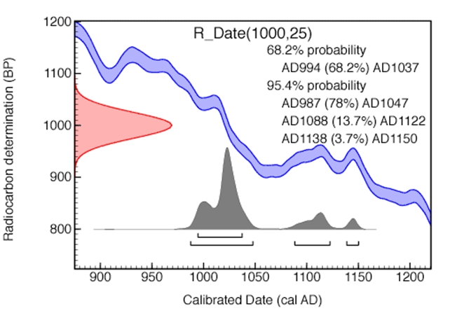
Downloaded from c14.arch.ox.ac.uk/embed.php ORAU May 2011
Dealing with one sample at a time is no longer a common occurrence, as frequently archaeologists will have a set of 14C results, related in some known way. In the simplest chronology construction setting, there would be a series of archaeological samples which are related through stratigraphy (which means that the relative ages of the samples from oldest to youngest can be defined). It may then be possible that some (or all) of the samples can be radiocarbon dated, and then in building the chronology, the 14C dates would need to be calibrated, whilst respecting the stratigraphic relationships. This step requires a more complex model but one which still has at its heart the model for calibrating a single 14C date.
In recent years within Archaeology there has been a major growth in the adoption of Bayesian models (Bayliss and Bronk Ramsay, 2004), characterized by the formal inclusion of the concept of ‘prior’ knowledge or beliefs into the modeling process.
Bayesian modeling and analysis has three key components, formally they are described as the prior, the likelihood and the posterior. Bayes theorem is used to define the posterior in terms of the likelihood (involving the data) and the prior (expressed in terms of the model parameters). The model parameters could for instance be the start and end date of an occupation layer or period, and these quantities will be described mathematically within the model.
First the prior captures expert archaeological knowledge about the parameters, so an archaeologist may be prepared to say that the start date can be no earlier than a particular event or time period, and that similarly the end date can be no later than another. An alternative approach would be to define the parameter of interest as the duration of occupation, so that the prior would provide a statement of the form “duration was greater than 20 years but less than 150 years”. Such statements would be written probabilistically (mathematically), so that in the latter case, one possibility would be to say that duration was equally likely to take any value between 20 and 150 years (or in other words to assume a Uniform distribution for duration). Considerable care is required in constructing the prior (Steir et al. 2000).
The likelihood is the next component and again is presented in probabilistic terms- here the observations are linked to the radiocarbon dates and the unknown parameters. The probability for each radiocarbon date is described given the unknown model parameters, and then these probabilities are generally multipled together to give the likelihood. The likelihood thus depends on the unknown parameters.
Finally, the posterior is then another probabilistic statement about the unknown parameters, but this time (unlike for the prior) the dates have also been used to define this statement, and in this way the archaeological knowledge is combined with the 14C measurements.
The Bayesian approach is probably best attempted in the context of calibration of radiocarbon ages using the readily available OxCal and BCal. For examples of application of the Bayesian approach in Scotland see Hamilton and Haselgrove (2009) and Hall et al. (2010).
General statistical modeling in Archaeology
More traditional statistical modeling, where there is no need for calibration, and where chronology construction is not the primary goal is also commonplace. Examples might include elemental compositions of glass shards, pottery descriptions (pattern, colour….).
Fundamentally, lying behind much of Statistics is the assumption of a population, from which a representative sample of individuals has been drawn. Statistical inference is the process whereby one generalises from the sample of observations to a wider population. The first step in defining a statistical model is to define a probability model that describes the variation in the attribute of interest within the population. A parameter of the probability model describes a population, while a statistic describes a sample. There are arguments concerning statistical models and the validity of the concept of population as applied in an archaeological context. Nonetheless, the idea of population is important, and linked to this is the idea of a probability model, which describes the variation of the variable of interest in the population. Commonly used probability models include the Normal and Poisson.
Hypothesis testing and confidence intervals
Hypothesis or significance testing is a formal method of statistical inference. The hypotheses are framed in terms of population parameters (such as the population mean or average).
Correlation and regression
When there are several variables (measured on the same artifact), then a common investigation concerns the relationships between the two. Such a question of interest would be answered using a) either Spearman or Pearson correlation coefficients (depending on distributional assumptions) and b) if it is considered that the value of one variable (response) is in fact determined by the other (explanatory), then one might consider building a regression model. This latter type of modeling structure can also be extended to the situation where there are potentially many explanatory variables.
Multivariate data
There are a variety of techniques including clustering, principal components analysis and discriminant analysis, commonly described as multivariate techniques, since they are applied to data sets where there are many artefacts, and on each artefact, there are a number of variables measured. Each specimen whether it be a pottery shard, glass fragment, or coin will have a number of measurements made on it (eg metallurgical analysis, or shape (length, breadth etc) or decoration). Since the measurements are made on a single specimen, they are likely to be related, so in this sense, we have an extension from the bivariate (two variable- correlation) case to the multivariate (many variable case).
Section 3 outlines the use of principal components and discriminate analysis which have been applied to elemental composition data of pottery.
See also More on Statistical Modelling Applications – just for the ScARF wiki!